This is Chapter 1 of the 10-part series The Physics & Engineering of Frontier LLM Inference. I announced the full series in Announcing the 10-Part Substack Series.
If you size an LLM serving fleet from parameter count alone, you will buy the wrong GPUs, miss the real bottleneck, and wonder why Tensor Cores sit idle while HBM runs at 100%.
Chapter 1 of my inference systems book starts from physics, not framework marketing. Autoregressive transformers split into two regimes with opposite hardware profiles: prefill (prompt processing) and decode (token generation). Prefill runs dense matrix-matrix multiplications and can saturate Tensor Cores. Decode runs matrix-vector multiplications one token at a time and streams the full weight tensor from HBM on every step. That asymmetry drives every serving decision that follows: batching, KV cache layout, chunked prefill, cluster sizing, and SLO design.
This article distills Chapter 1 of my inference systems book, The Physics of LLM Inference (2026 Edition, to be published soon). The free preview covers the roofline model, the prefill/decode split, and the latency taxonomy every SRE should instrument. Paid subscribers get VRAM accounting, chunked prefill mechanics, continuous batching and PagedAttention, cluster sizing code, and a discrete-event simulator you can run locally.
The roofline model (Williams et al., 2009) maps attainable FLOP/s to operational intensity I, measured as total FLOPs divided by bytes moved across the memory bus:
P_attainable = min(P_peak, I × BW_mem)
The ridge point Iridge = Ppeak / BW_mem is where compute and bandwidth ceilings meet. Below the ridge, kernels are memory-bandwidth bound. Above it, they are compute bound.
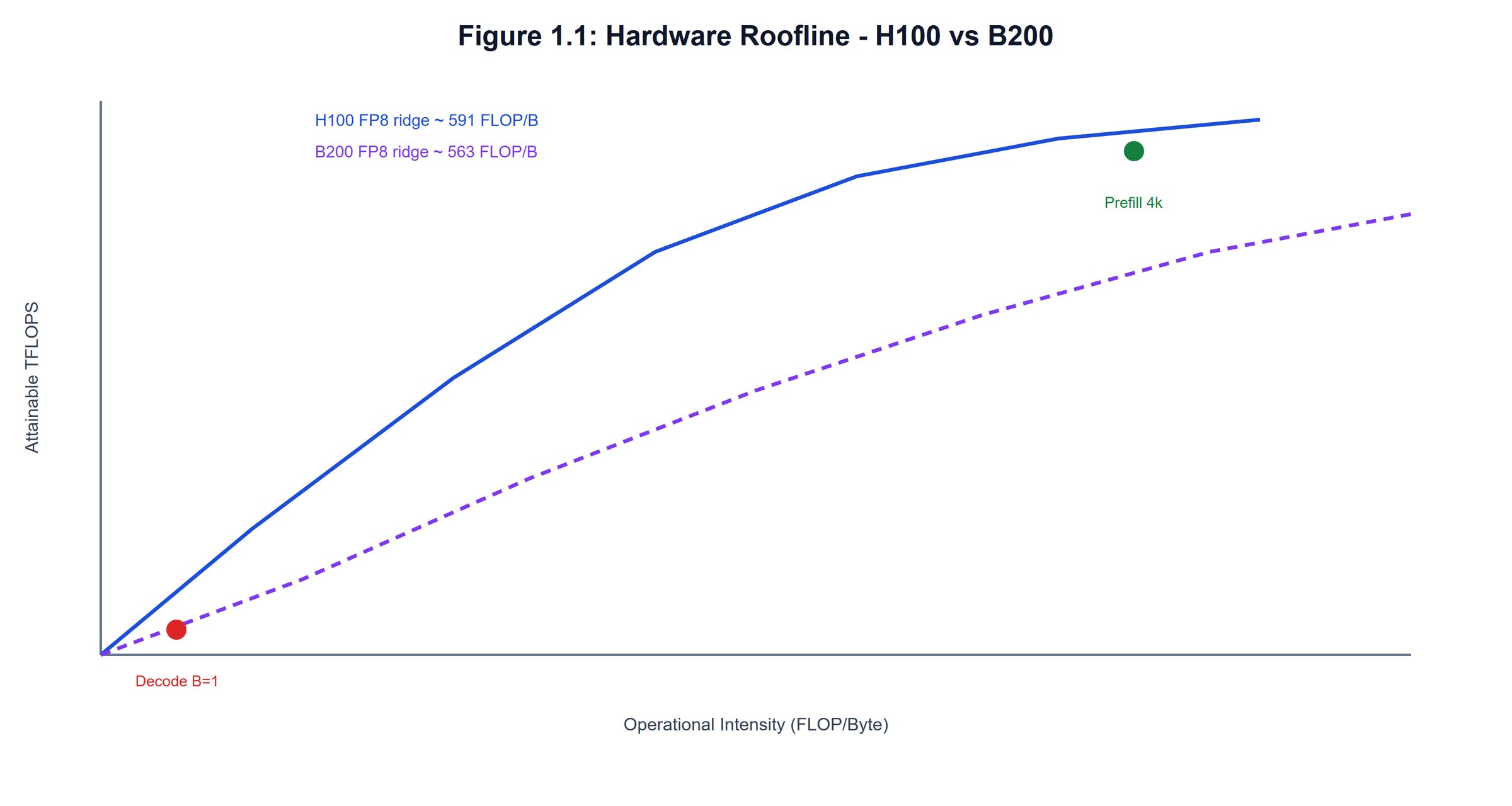
Figure 1.1 places decode and prefill on that chart for Hopper H100 and Blackwell B200 class hardware. Decode at B=1 sits far left of the ridge. Prefill at 4k tokens sits on the compute side.
Figure 1.1: Hardware Roofline - H100 vs B200
Table 1.1 lists ridge points for frontier accelerators. Compute has scaled faster than HBM bandwidth across generations, which pushes the ridge rightward and makes batching more important, not less.
Table 1.1: Frontier Accelerator Ridge Points (2026)
On an H100 SXM5 in FP8 (1,979 TFLOPS peak, 3.35 TB/s HBM3), I_ridge ≈ 591 FLOP/byte. Single-stream decode at I ≈ 1.5 FLOP/byte delivers under 0.3% of peak Tensor Core throughput. That is not a software bug. It is the physics of GEMV at scale.
The escape hatch is batching. When B independent decode streams share one weight load, intensity scales approximately as I(B) ≈ (2 / S_weight) × B. For FP8 weights, B ≈ 296 streams would be required to hit the H100 ridge in theory. Production systems rarely run that hot because KV cache memory and latency SLOs cap batch size first.
Training optimizes for throughput over large static batches. Inference optimizes for latency under variable concurrency. A vision model runs one forward pass. A generative LLM runs one forward pass per output token, and the work profile changes between the first token and every token after it.
During prefill, the engine processes the full prompt in parallel. Operational intensity lands in the 150–450 FLOP/byte range on modern accelerators. Tensor Cores stay busy.
During decode, each active sequence contributes one token vector per step. The forward pass degrades into GEMVs. Intensity drops to roughly 1–2 FLOP/byte at batch size B=1. The GPU loads tens of gigabytes of weights to perform a comparatively tiny amount of arithmetic. Over 99% of cycle time can stall on memory transfers.
Figure 1.2 names the split that every capacity plan must respect: prefill governs Time to First Token (TTFT); decode governs Inter-Token Latency (ITL), also called Time Per Output Token (TPOT).
Figure 1.2: Prefill vs Decode Execution Waterfall
Figure 1.3 shows why register files and SRAM cannot rescue single-stream decode: the full model still transits HBM every token.
Figure 1.3: GPU Memory Hierarchy Ladder
Consider a 70B model in FP8 (70 GB weights) on an H100 (3.35 TB/s HBM3):
Weight transfer time: 70 GB / 3.35 TB/s ≈
20.9 msTensor Core compute for ~140 GFLOPs: ≈
0.07 ms
Memory accounts for 99.66% of step time. Any optimization that does not reduce bytes moved per token (quantization, batching, speculative decoding with acceptance, KV compression) fights uphill against this ratio.
Production teams instrument three clocks:
TTFT = Tqueue + Tprefixlookup + Tprefillcompute + Tsample
Queue wait, radix-tree prefix cache hits, dense prefill GEMMs, and sampling overhead all land before the first visible token.
ITL (or TPOT) is the gap between consecutive token emissions. Interactive UIs need ITL below 30–50 ms (20–33 tokens/sec). Background agent workflows can relax to 80–120 ms to run larger batches.
End-to-end latency for M generated tokens: TE2E = TTFT + (M - 1) × ITLmean. Tail percentiles (P95/P99 ITL) matter as much as means when prefill and decode share SMs.
This is where the free preview ends. Paid subscribers get VRAM accounting (weights, KV cache, activations, runtime buffers), chunked prefill and piggybacking math, Orca continuous batching and PagedAttention, tensor-parallel interconnect costs, a cluster sizing engine, and a discrete-event simulator with runnable Python. To unlock the full treatise, subscribe now for 50% off annual membership.